General Vignette

Welcome to testComplexity!

This section has been written with the intent to provide the user a general introduction to the features and functionality of the package via a set of textual elucidations and with an example discussed throughout for each of the user-oriented functions.

Brief Overview

As can be guessed from the name itself, this package provides a suite of functions to systematically test the asymptotic complexities of R functions/algorithms, where the term “complexity” here refers to the time complexity, as per the initial idea. (for instance, the logo is based on relevance with time!)

Features

Going by the base objectives stated here, this package provides:

A function for quantifying the empirical time complexity of any R expression.
A time complexity classifying function which operates on the result (a data frame) of the previous function.
Testing functions, to test for an expected time complexity class directly.

In addition to these, a few more features have been implemented:

A function for quantifying memory allocations and one for subsequently classifying the space/memory complexity.
Plotting functions for both time and memory cases.
A complexity classifier for generalized use in asymptotic trend classification among any two parameters, not being restricted to time/memory cases.

Usage Notes

Based on whether the user has an idea of the complexity class the input algorithm falls in, two scenarios are possible:

The complexity class of the algorithm is not known, or diagnostic tests to estimate it have not been performed yet. In this case, the user could directly use the quantifiers and complexity classifiers to obtain the asymptotic complexity class.
The complexity class is known via theoretical proof/empirical observation. For this case, the user can directly proceed to use the testers for verifying the theoretically-derived/empirically-obtained result, apart from using the previous method.

Note that the worst-case complexity class is currently set to quadratic. Cubic and exponential classes were initially thought of to be included, but since a \(O(N^2)\) approach is the limit in practically used algorithms, subsequently higher complexity classes were discarded.

If the estimated complexity class turns out to be quadratic, its an indicator that the algorithm could do with a better approach, so as to minimize the computational resources (time/memory).

In such situations, the user may as well want to think of ways to reduce the time complexity, in which case the aforementioned functions will be helpful to continuously give feedback (via re-runs) for each improvement that the user thinks could make a difference in the complexity trend. This in turn could potentially lead to improvements in code performance, if such feedback-based optimizations are implemented in order to achieve better computational efficiency.

Examples

To demonstrate the functionality of our package, I’ll be taking the function PeakSegPDPA from the PeakSegOptimal package as an example for each of the functions stated below. Note that it is empirically observed to be a log-linear time and memory algorithm, or the expected complexity classes for both time and memory cases is \(O(NlogN)\) for input size \(N\). This fact here is essential to know before-hand as you’ll see¹ that testComplexity’s functions obtain the same result, demonstrating its accuracy.

Function Categories

Based on the different aspects of functionality, the functions in this package can be grouped into four distinct categories:

Quantifiers

These are the quantifying functions which compute the empirical benchmarks for runtimes (via the asymptoticTimings() function) and memory allocations (via the asymptoticMemoryUsage() function) against allotted data sizes. For user convenience, a few points have been taken note of with respect to the parameters:

The user-supplied algorithm is ideally accepted as an expression, which would be a function that scales with N (as a parameter) so as to comply with the general notation of N resembling the input size when we refer to asymptotic complexity classes (such as \(O(N)\) denoting the linear variant, or a linear asymptotic trend in \(N\)). The values which N can take are seperately specified by the vector/set of user-provided values for the argument data.sizes.
Parameters such as max.bytes and max.seconds are introduced to put a desirable restriction on the time invested and memory allocated respectively, thereby saving resources (time/memory) for the otherwise possible further computation once the limit has been breached. The default values have been set taking into account the correct prediction for different test-cases, and should enact as an appropriate threshold for most algorithms.

The only requirement for the user is to be able to identify the parameter in his/her own function/algorithm which can scale asymptotically for different data sizes, or in simple terms the parameter which can contain different values and the function’s resource utilization varies depending on that. (which is fairly easy to figure out and is expected from the user)

To demonstrate the working, let us consider the example function PeakSegOptimal::PeakSegPDPA() and its parameters:

count.vec: It should be an integer vector of count data.
weight.vec: Its a numeric vector of positive weights, which would be computed via count.vec automatically from the default assignment. (doesn’t need to be specified)
max.integer: Maximum number of integer segments, which should be >=2 in value.

From the list of parameters above, the count.vec parameter is the one which when adjusted with higher values results in greater resource (time/memory) consumption, scaling asymptotically. Now in accordance with the first point mentioned above, we need to have that input vector of data as a function of N, which is relatively straight-forward depending on what type of data the function operates on. As per the function’s description, it states that the algorithm computes optimal changepoint models using the Poisson likelihood for non-negative count data, which means we need to create a vector of poisson data in N, which is as simple as:

data.vec = rpois(N, 1)

Now we simply emplace that function with its parameters for our expression argument in asymptoticTimings() and asymptoticMemoryUsage(), along with suitable data sizes to obtain the quantified timings/memory allocations respectively:

df.time <- asymptoticTimings(e = PeakSegOptimal::PeakSegPDPA(count.vec = data.vec, max.segments = 3L), data.sizes = 10^seq(1, 4, by = 0.1))
data.table::data.table(df.time)
#>       Timings Data sizes
#>  1:    248701         10
#>  2:    120302         10
#>  3:    125701         10
#>  4:    133301         10
#>  5:    146500         10
#> ---                     
#> 696: 405597501      10000
#> 697: 408335001      10000
#> 698: 338544401      10000
#> 699: 404081901      10000
#> 700: 399575501      10000

df.memory <- asymptoticMemoryUsage(PeakSegOptimal::PeakSegPDPA(count.vec = data.vec, max.segments = 3L), data.sizes = 10^seq(1, 4, by = 0.1))
data.table::data.table(df.memory)
#>    Memory usage Data sizes
#> 1:         6256   10.00000
#> 2:         7024   12.58925
#> 3:         7432   15.84893
#> 4:         8560   19.95262
#> 5:         9496   25.11886
#> --- 
#> 25:       447792 2511.88643
#> 26:       562336 3162.27766
#> 27:       706512 3981.07171
#> 28:       887792 5011.87234
#> 29:      1116240 6309.57344

If the seperate use of N in the step-wise argument construction for the above demonstration seems confusing, one can simply pass the parameters directly like count.vec = rpois(N, 1) (avoiding use of data.vec) or just rpois(N, 1) (passing arguments in order).

Now that we have obtained our benchmarked data (consisting of runtimes and memory allocations) in a convienent data.frame format, we can proceed to find out the complexity class as demonstrated below.

Complexity Classifiers

These are the complexity classification functions which internally use different stochastic procedures (such as cross-validation on different glm models, as derived from GuessCompx) to compute the complexity class for the user-provided algorithm via a best model match. Using them is relatively quite simple, as one just needs to pass the data frame obtained from the quantifiers to the appropriate complexity classifier.

As an example, consider the data frames we obtained above for our function PeakSegOptimal::PeakSegPDPA() and pass them onto the complexity classifiers asymptoticTimeComplexityClass() and asymptoticMemoryComplexityClass() for time and memory cases respectively:

asymptoticTimeComplexityClass(df.time)
#> [1] "loglinear"

asymptoticMemoryComplexityClass(df.memory)
#> [1] "loglinear"

The resulting complexity classes turned out to be log-linear for both time and memory cases, (coincidentally for this function they are the same) which are exactly¹ the expected complexity classes.

Note that you can chain the quantifiers with them, or call them and operate on their returned data frames directly:

asymptoticTimeComplexityClass(asymptoticTimings(e = PeakSegOptimal::PeakSegPDPA(count.vec = data.vec, max.segments = 3L), data.sizes = 10^seq(1, 4, by = 0.1)))
#> [1] "loglinear"
asymptoticMemoryComplexityClass(asymptoticMemoryUsage(PeakSegOptimal::PeakSegPDPA(count.vec = data.vec, max.segments = 3L), data.sizes = 10^seq(1, 4, by = 0.1)))
#> [1] "loglinear"

Furthermore, if the user wants to classify the asymptotic trend between two custom parameters (which are not subject to being only runtimes/memory-allocations), they can use the asymptoticComplexityClass() function which as intended, computes the complexity class based on the trend followed between any two parameters of user-provided data which are contained in a data frame.

The function accepts a data frame along with the two columnar parameters which the user needs to specify (as to which designates the output metric and which designates the data sizes, or something to relatively measure the trend against).

Note that since the computed data is already prevalent in the specified output parameter column of the data frame, we don’t need to use our quantifying functions or perform any benchmarks.

As a recurring example, consider passing the column names ‘Timings’ and ‘Data sizes’ along with the data frame returned by the time quantifier: (it consists of those two columns)

asymptoticComplexityClass(df, output.size = "Timings", data.size = "Data sizes")
#> [1] "loglinear"

As expected, it classifies the correct complexity just like asymptoticTimeComplexityClass() did, as because the underlying complexity classification procedure is same. Its just that the parameters are customizable, which leads to a wider use-case scenario than just classifying the trend for time/memory cases.

Testers

These are the functions used to test the user-provided algorithm against an expected complexity class. They can be used to verify the theoretically derived or empirically observed complexities either directly or by disregarding the remaining complexity classes to prove the same via contradiction.

There are three surface level functions meant for the user, namely expect_linear_time(), expect_loglinear_time() and expect_quadratic_time(), all of which as their respective names suggest can be used to test an algorithm against the named complexity class. If the algorithm shows the expected complexity, it doesn’t throw any error. Otherwise a complexity mismatch error is thrown with a traceback from the calling point to the inner functions. Other complexity classes such as constant and log were not taken into account for the moment since these three tend to cover all cases for our test functions. Also note that variants of these functions for dealing with memory have not been implemented since they are not a part of the base objective plus for the fact that the memory quantifier deals with memory allocations at the moment, and might not be fit for all cases.

These functions accept the same parameters as the ones used in asymptoticTimings(), so they provide a suitable alternative to the user in place of using the time quantifier and complexity classifier in conjunction.

As an example, lets take our function PeakSegPDPA() and test it against different complexity classes:

expect_loglinear_time({
data.vec <- rpois(N, 1)
PeakSegOptimal::PeakSegPDPA(data.vec, max.segments = 3L)}, data.sizes = 10^seq(1, 4, by = 0.5))
# or:
# expect_loglinear_time(PeakSegOptimal::PeakSegPDPA(rpois(N, 1), max.segments = 3L), data.sizes = 10^seq(1, 4, by = 0.5))
#> [1] "loglinear"

The above function throws no error, which means that our algorithm does follow a log-linear trend. On the other hand, if we test for the same against the linear or quadratic variants, we would get errors: (as expected)

expect_linear_time({
data.vec <- rpois(N, 1)
PeakSegOptimal::PeakSegPDPA(data.vec, max.segments = 3L)}, data.sizes = 10^seq(1, 4, by = 0.5))
#> [1] "loglinear"
#> Error: Complexity mismatch: Expected linear complexity, instead of the predicted loglinear complexity from asymptoticTimeComplexityClass(timings.df).

expect_quadratic_time({
data.vec <- rpois(N, 1)
PeakSegOptimal::PeakSegPDPA(data.vec, max.segments = 3L)}, data.sizes = 10^seq(1, 4, by = 0.5))
#> [1] "loglinear"
#> Error: Complexity mismatch: Expected quadratic complexity, instead of the predicted loglinear complexity from asymptoticTimeComplexityClass(timings.df).

The call stack (sequence of calls that lead to the error) is returned via a call to traceback() as well, although the user doesn’t need to exemplify the verification through that, since the error message itself clearly states the inequality between the expected and predicted complexity classes, which can be used to prove by contradiction.

Plotters

These functions are for plotting the metrics returned by the quantifiers, in case the user still prefers to diagnose the obtained complexity result via the traditional method, i.e. with a visual representation of the benchmarked data.

Considering the columns from the data frames returned by the quantiftying functions, the user can create plots for ‘Timings’ vs ‘Data sizes’ via plotTimings() and for ‘Memory usage’ vs ‘Data sizes’ via plotMemoryUsage():

# Plot the trend between benchmarked timings and data sizes:
df.time <- asymptoticTimings(PeakSegOptimal::PeakSegPDPA(rpois(N, 1), max.segments = 3L), data.sizes = 10^seq(1, 4, by = 0.5))
time.plot <- plotTimings(df.time, titles = list("Timings plot", "PeakSegOptimal::PeakSegPDPA"), labels = list("Data size", "Runtime (in nanoseconds)"), point.color = "black", line.color = "#9c9494", point.size = 1.6, line.size = 1.2)

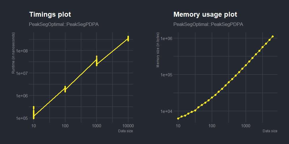
# Plot the trend between computed memory allocations vs data sizes:
df.memory <- asymptoticMemoryUsage(PeakSegOptimal::PeakSegPDPA(rpois(N, 1), max.segments = 3L), data.sizes = 10^seq(1, 4, by = 0.1))
memory.plot <- plotMemoryUsage(df.memory, titles = list("Memory usage plot", "PeakSegOptimal::PeakSegPDPA"), labels = list("Data size", "Memory size (in bytes)"), point.alpha = 1, line.alpha = 0.8, point.color = "#000000", line.color = "#9c9494", point.size = 2, line.size = 1)

gridExtra::grid.arrange(time.plot, memory.plot, ncol = 2)

Themes can be directly appended to the ggplot object returned by the plotters:

time.plot <- plotTimings(df.time, titles = list("Timings plot", "PeakSegOptimal::PeakSegPDPA"), labels = list("Data size", "Runtime (in nanoseconds)"), point.color = "#ffec1b", line.color = "#ffec1b", point.size = 1.5, line.size = 1.1)
memory.plot <- plotMemoryUsage(df.memory, titles = list("Memory usage plot", "PeakSegOptimal::PeakSegPDPA"), labels = list("Data size", "Memory size (in bytes)"), point.alpha = 1, line.alpha = 0.8, point.color = "#ffec1b", line.color = "#ffec1b", point.size = 2, line.size = 1)

themed.time.plot <- time.plot + hrbrthemes::theme_ft_rc()
themed.memory.plot <- memory.plot + hrbrthemes::theme_ft_rc()

gridExtra::grid.arrange(themed.time.plot, themed.memory.plot, ncol = 2)

For the users relatively new to such diagnostic plots for benchmarking/profiling, it might seem hard to figure the trend just by looking at such individual plots. By testing with more functions, the graphical trends for the complexity classes become more clearly distinguishable over time. But for a quicker alternative, comparison plots can be created. For instance, the function we considered in our examples here (PeakSegPDPA()) follows a log-linear trend (as proven above), so we can consider another function with either a lower or higher complexity class, and test for our function’s plot-line to be above or lower respectively. As an example, consider comparing the trends in timings versus data sizes of PeakSegOptimal::PeakSegPDPA() with the function PeakSegDP::cDPA(), which is found to be quadratic in nature:

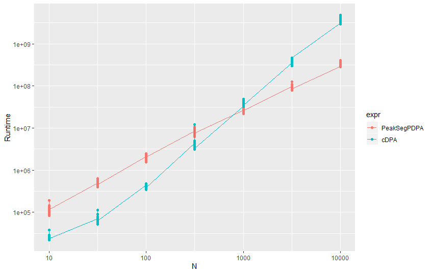
By observing the above figure, the user can tell that PeakSegPDPA() would fall in a lower complexity class in comparison to cDPA() (provided we know the later follows a quadratic trend), with the difference scaling asymptotically. However, it might not be clear whether it falls in the log-linear or linear zone by just looking at this comparison, (visually diagnosing a distinct complexity class from benchmarked data is difficult) which is the reason why our package thrives to provide a much more convenient alternative via the use of testers and complexity classifiers (operating on data supplied from the quantifiers).

Without this added convenience or a good visual diagnosis capability, the user may need to prepare a seperate comparison plot considering all the complexities (with glm-mapped values for instance) along with the required algorithm to figure the resultant complexity class. As an example, such a plot for our taken algorithm with regression based plotlines (considering runtime values at the extremities) would look like:

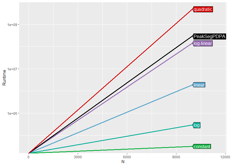
It is clear that our algorithm PeakSegPDPA() follows a log-linear asymptotic trend as can be observed from the above plot, with the plotline for the function being in close proximity to (or having the least deviation from) the log-linear line.

That sums up the functionality offered by testComplexity 0.1.0. For more examples, please check the articles section from the navigation bar of the website.

Anirban Chetia

2020-08-29