Asymptotic Complexity Testing Framework • testComplexity

Abstract

R package developers currently use ad-hoc tests of asymptotic computational complexity via empirical timings of functions and visual diagnostic plots. However, there is no framework in R for systematically testing the empirical computational complexity of functions, which tends to be a problem because such a testing framework could be essential for identifying big speed gains in R code as well. In response to this, testComplexity provides a suite of functions that will be useful for testing and thereby improving the speed of various algorithms/functions in R.

Since algorithms are used in every sphere of research, this package potentially caters to all sorts of R-users, following different fields of study. Currently, it is being tested on changepoint detection, constrained optimal segmentation/partitioning algorithms plus a few regular ones such as substring and gregexpr.

Setup

Use devtools or remotes to fetch the package from the GitHub repository:

if(!require(devtools)) install.packages("devtools")
devtools::install_github("Anirban166/testComplexity")

if(!require(remotes)) install.packages("remotes")
remotes::install_github("Anirban166/testComplexity")

Functional Flow

__________________ R Files _______________________________________ Additional Details _____________________________
testComplexity                              @ returns              @ type                    @ commit-branch(es)
├──> asymptoticTimings                    : data.frame             timings quantifier        master
│    ├──> asymptoticTimeComplexityClass   :   ├──> string          ↑ complexity classifier   master
│    └──> plotTimings                     :   └──> ggplot object   ↑ plotter                 master/Plotfunc
│
├──> asymptoticMemoryUsage                : data.frame             memory-usage quantifier   Memtest
│    ├──> asymptoticMemoryComplexityClass :   ├──> string          ↑ complexity classifier   Memtest
│    └──> plotMemoryUsage                 :   └──> ggplot object   ↑ plotter                 Memtest/Plotfunc
│
├──> asymptoticComplexityClass            : string                 complexity classifier     Generalizedcomplexity
│    └──> asymptoticComplexityClassifier  :   ↑ string             ↑ complexity classifier   Generalizedcomplexity
│
├──> expect_complexity_class              : -/-                    test function             Testfunc
│    └──> expect_time_complexity          : -/-                    ↑  test function          Testfunc
│         ├──> expect_linear_time         : -/-                    ↑↑ test function          Testfunc
│         ├──> expect_loglinear_time      : -/-                    ↑↑ test function          Testfunc
│         └──> expect_quadratic_time      : -/-                    ↑↑ test function          Testfunc
│
└──> testthat
     ├──> testsfortestComplexity                                   unit-tester               All branches
     ├──> testsforConstrainedchangepointmodelalgos                 unit-tester               Testfunc
     └──> testsforRegularfunctions                                 unit-tester               Testfunc
____________________________________________________________________________________________________________________

Usage

To get started, please check the general vignette which highlights all the features, enlists the different types of function categories existent in the package and describes the functionality offered by the underlying user-oriented functions via a set of textual elucidations with one example taken to be discussed throughout for each of them.

For a quick overview of the main functionality (obtaining quantified benchmarks and subsequently computing the time/memory complexity class), please check the examples below.

To obtain the benchmarked timings/memory-allocations against specified data sizes, pass the required algorithm as a function of N to asymptoticTimings()/asymptoticMemoryUsage():

library(data.table)
# Example 1 | Applying the bubble sort algorithm to a sample of 100 elements: (expected quadratic time complexity & constant memory complexity)
bubble.sort <- function(elements.vec) { 
  n <- length(elements.vec)
  for(i in 1:(n - 1)) {
    for(j in 1:(n - i)) {
      if(elements.vec[j + 1] < elements.vec[j]) { 
        temp <- elements.vec[j]
        elements.vec[j] <- elements.vec[j + 1]
        elements.vec[j + 1] <- temp
      }
    }
  }
  return(elements.vec)
}

df.bubble.time <- asymptoticTimings(bubble.sort(sample(1:100, N, replace = TRUE)), data.sizes = 10^seq(1, 3, by = 0.5))
data.table(df.bubble.time)
      Timings Data sizes
  1:    91902         10
  2:    39402         10
  3:    34701         10
  4:    33101         10
  5:    33201         10
 ---
496: 64490501       1000
497: 59799101       1000
498: 63452200       1000
499: 62807201       1000
500: 59757102       1000

df.bubble.memory <- asymptoticMemoryUsage(bubble.sort(sample(1:100, N, replace = TRUE)), data.sizes = 10^seq(1, 3, by = 0.1))
data.table(df.bubble.memory)
    Memory usage Data sizes
 1:        87800   10.00000
 2:         2552   12.58925
 3:         2552   15.84893
 4:         2552   19.95262
 5:         2552   25.11886
 ---
17:         7472  398.10717
18:         8720  501.18723
19:        10256  630.95734
20:        12224  794.32823
21:        14696 1000.00000

# Example 2 | Testing PeakSegPDPA, an algorithm for constrained changepoint detection: (expected log-linear time and memory complexity)
data.vec <- rpois(N, 1)
df.PDPA.time <- asymptoticTimings(PeakSegOptimal::PeakSegPDPA(count.vec = data.vec, max.segments = 3L), data.sizes = 10^seq(1, 4, by = 0.1))
&data.table(df.PDPA.time)
       Timings Data sizes
  1:    248701         10
  2:    120302         10
  3:    125701         10
  4:    133301         10
  5:    146500         10
 ---
696: 405597501      10000
697: 408335001      10000
698: 338544401      10000
699: 404081901      10000
700: 399575501      10000

df.PDPA.memory <- asymptoticMemoryUsage(PeakSegOptimal::PeakSegPDPA(count.vec = data.vec, max.segments = 3L), data.sizes = 10^seq(1, 4, by = 0.1))
data.table(df.PDPA.memory)
    Memory usage Data sizes
 1:         6256   10.00000
 2:         7024   12.58925
 3:         7432   15.84893
 4:         8560   19.95262
 5:         9496   25.11886
 ---
25:       447792 2511.88643
26:       562336 3162.27766
27:       706512 3981.07171
28:       887792 5011.87234
29:      1116240 6309.57344

To estimate the corresponding time/memory complexity class, pass the obtained data frame onto asymptoticTimeComplexityClass()/asymptoticMemoryComplexityClass():

# Example 1 | Applying the bubble sort algorithm to a sample of 100 elements: (expected quadratic time complexity & constant memory complexity)
asymptoticTimeComplexityClass(df.bubble.time)
[1] "quadratic"
asymptoticMemoryComplexityClass(df.bubble.memory)
[1] "constant"

# Example 2 | Testing PeakSegPDPA, an algorithm for constrained changepoint detection: (expected log-linear time and memory complexity)
asymptoticTimeComplexityClass(df.PDPA.time)
[1] "loglinear"
asymptoticMemoryComplexityClass(df.PDPA.memory)
[1] "loglinear"

Combine the functions if you only require the complexity class:

# Example 3 | Testing the time complexity of the quick sort algorithm: (expected log-linear time complexity)
asymptoticTimeComplexityClass(asymptoticTimings(sort(sample(1:100, N, replace = TRUE), method = "quick" , index.return = TRUE), data.sizes = 10^seq(1, 3, by = 0.5)))
[1] "loglinear"

# Example 4 | Allocating a square matrix (N*N dimensions): (expected quadratic memory complexity)
asymptoticMemoryComplexityClass(asymptoticMemoryUsage(matrix(data = N:N, nrow = N, ncol = N), data.sizes = 10^seq(1, 3, by = 0.1)))
[1] "quadratic"

Check this screencast for a demonstration of time complexity testing on different sorting algorithms over a test session.

Plotting

For obtaining a visual description of the trend followed between runtimes/memory-usage vs data sizes so as to diagnose the complexity result(s), simple plots can be crafted. They are roughly grouped into:

Single Plots
Individual plots can be obtained by passing the data frame returned by the quantifying functions to plotTimings()/plotMemoryUsage() for time/memory cases respectively:

# Timings plot for PeakSegDP::cDPA
df <- asymptoticTimings(PeakSegDP::cDPA(rpois(N, 1), rep(1, length(rpois(N, 1))), 3L), data.sizes = 10^seq(1, 4))
plotTimings(df.time, titles = list("Timings", "PeakSegDP::cDPA"), line.color = "#ffec1b", point.color = "#ffec1b", line.size = 1, point.size = 1.5)
# Equivalent ggplot object:
df <- asymptoticTimings(PeakSegDP::cDPA(rpois(data.sizes, 1), rep(1, length(rpois(data.sizes, 1))), 3L), data.sizes = 10^seq(1, 4))
ggplot(df, aes(x = `Data sizes`, y = Timings)) + geom_point(color = ft_cols$yellow, size = 1.5) + geom_line(color = ft_cols$yellow, size = 1) + labs(x = "Data sizes", y = "Runtime (in nanoseconds)") + scale_x_log10() + scale_y_log10() + ggtitle("Timings", "PeakSegDP::cDPA") + hrbrthemes::theme_ft_rc()

# Memory Usage plot for PeakSegDP::cDPA
df <- asymptoticMemoryUsage(PeakSegDP::cDPA(rpois(N, 1), rep(1, length(rpois(N, 1))), 3L), data.sizes = 10^seq(1, 6, by = 0.1))
plotMemoryUsage(df.memory, titles = list("Memory Usage", "PeakSegDP::cDPA"), line.color = "#ffec1b", point.color = "#ffec1b", line.size = 1, point.size = 2)
# Equivalent ggplot object:
ggplot(df, aes(x = `Data sizes`, y = `Memory usage`)) + geom_point(color = ft_cols$yellow, size = 2) + geom_line(color = ft_cols$yellow, size = 1) labs(x = "Data sizes", y = "Memory usage (in bytes)") + scale_x_log10() + scale_y_log10() + ggtitle("Memory Usage", "PeakSegDP::cDPA") + hrbrthemes::theme_ft_rc()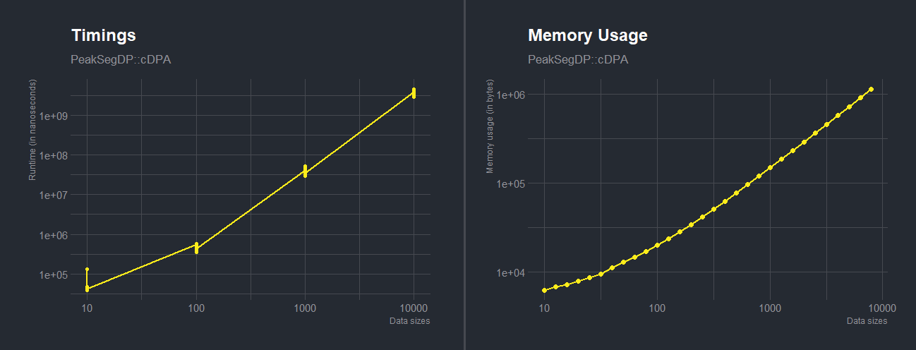

Comparison Plots
In order to visually compare different algorithms based on the benchmarked metrics returned as a data frame by the quantifiers, one can appropriately add a third column (to help distinguish by aesthetics based on it) with a unique value for each of the data frames, combine them using an rbind() and then plot the resultant data frame using suitable aesthetics, geometry, scale, labels/titles etcetera via a ggplot:

df.substring <- asymptoticTimings(substring(paste(rep("A", N), collapse = ""), 1:N, 1:N), data.sizes = 10^seq(1, 4, by = 0.5))
asymptoticTimeComplexityClass(df.substring)
[1] "linear"
df.PeakSegPDPA <- asymptoticTimings(PeakSegOptimal::PeakSegPDPA(rpois(N, 1),rep(1, length(rpois(N, 1))), 3L), data.sizes = 10^seq(1, 4, by = 0.5), max.seconds = 1)
asymptoticTimeComplexityClass(df.PeakSegPDPA)
[1] "loglinear"
df.cDPA <- asymptoticTimings(PeakSegDP::cDPA(rpois(N, 1), rep(1, length(rpois(N, 1))), 3L), data.sizes = 10^seq(1, 4, by = 0.5), max.seconds = 5)
asymptoticTimeComplexityClass(df.cDPA)
[1] "quadratic"
df.gregexpr <- asymptoticTimings(gregexpr("a", paste(collapse = "", rep("ab", N)), perl = TRUE), data.sizes = 10^seq(1, 4, by = 0.5))
asymptoticTimeComplexityClass(df.gregexpr)
[1] "linear"
df.fpop <- asymptoticTimings(fpop::Fpop(rnorm(N), 1), data.sizes = 10^seq(1, 4, by = 0.5))
asymptoticTimeComplexityClass(df.fpop)
[1] "loglinear"
df.opart <- asymptoticTimings(opart::opart_gaussian(rnorm(N), 1), data.sizes = 10^seq(1, 4, by = 0.5))
asymptoticTimeComplexityClass(df.opart)
[1] "quadratic"

df.substring$expr = "substring"
df.PeakSegPDPA$expr = "PeakSegPDPA"
df.cDPA$expr = "cDPA"
df.gregexpr$expr = "gregexpr"
df.fpop$expr = "fpop"
df.opart$expr = "opart"

plot.df <- rbind(df.substring, df.PeakSegPDPA, df.cDPA, df.gregexpr, df.fpop, df.opart)
ggplot(plot.df, aes(x = `Data sizes`, y = Timings)) + geom_point(aes(color = expr)) + geom_line(aes(color = expr)) + labs(x = "Data sizes", y = "Runtime (in nanoseconds)") + scale_x_log10() + scale_y_log10() + ggtitle("Timings comparison plot", subtitle = "Linear vs Log-linear vs Quadratic complexities") + ggthemes::theme_pander()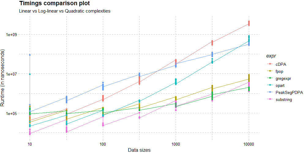

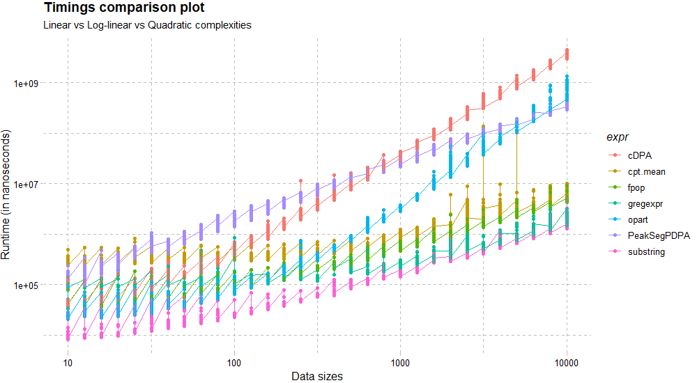
Feel free to include more functions and increase the number of data sizes for a more comprehensive outlook:

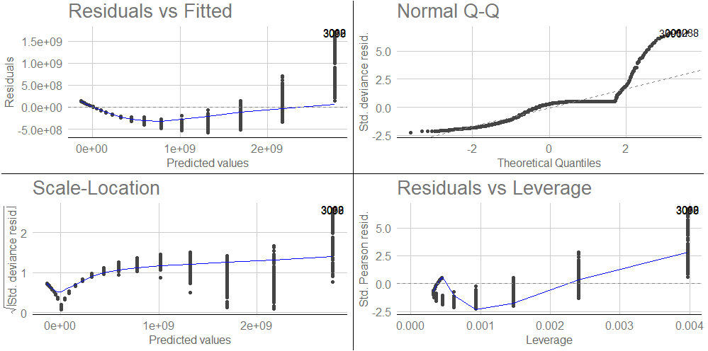
Generalized Linear Model based Plots
ggfortify, an extension of ggplot2, can be used to produce diagnostic plots for generalized linear models with the same formulae as used in the complexity classification functions:

library(ggfortify)
df <- asymptoticTimings(PeakSegDP::cDPA(rpois(N, 1), rep(1, length(rpois(N, 1))), 3L), data.sizes = 10^seq(1, 4 by = 0.1))
glm.plot.obj <- glm(Timings~`Data sizes`, data = df)
ggplot2::autoplot(stats::glm(glm.plot.obj)) + ggthemes::theme_gdocs()

Benchmarking

Among a few options,

microbenchmark::microbenchmark() is used to compute the benchmarks to obtain the time results in testComplexity::asymptoticTimings(), for the added convenience of having the benchmarked results as a data frame plus for the precision or time scale it produces the results on. (usually in nanoseconds, as can be found from here)
bench::bench_memory() is used to compute the allocated memory size in order to obtain the memory use metrics in testComplexity::asymptoticMemoryUsage().

Testing

Functions
A complexity-wise ordered list of the current set of functions taken into consideration for testing our functionality can be found here.
A dedicated vignette-based article for each can be found via the ‘Articles’ section, accessible from this website’s navigation bar at the top.
Unit Testing
Test cases for testComplexity functions via testthat package can be found here.
Code Coverage
Tested using covr::package_coverage() both locally and via codecov, with 100% coverage attained.
OS Support
Windows is the native OS this package is developed and tested on, but in addition to that, RCMD checks are run on latest versions of Ubuntu and MacOS as well.
Note that the use of bench::bench_memory() overcomes the drawback of windows-only OS limitation for memory complexity testing as observed in GuessCompx::CompEst() since it successfully runs on other operating systems.

Abstract

Setup

Functional Flow

Usage

Plotting

Benchmarking

Testing

Blog Posts

Links

License

Developers

Dev status