Skewness and Kurtosis both pertain to the ‘tailedness’ of the probability distribution of a real-valued random variable. They ordinally describe the shape of a probability distribution, giving different ways of quantifying it for a theoretical distribution and corresponding ways of estimating it from a sample of a population.
In this post, I have covered their computation (along with other statistical parameters involved in their formulae such as mean, standard deviation, median, etc.) on a sample size of 1000 consisting of random variables in the range of -100 to 100 (both size and range adjustable) via a C++ program.
Formulae used:
Here x̅ is the mean, s is the standard deviation, and N is the number of data points or our sample size. The above formula for skewness is referred to as the Fisher-Pearson coefficient of skewness. (Reference)
Following an alternative formula, the Pearson 2 skewness coefficient is defined as:
ȳ here is the median.
Additionally, since the kurtosis for a standard normal distribution is three, you may find the formula for kurtosis above appended with a negative three. (referred to as the excess)
My implementation:
#include <iostream>
#include <random>
#include <cmath>
#include <vector>
#include <algorithm>
// Defining an alias for the required data type: (Avoid using integer since decimal figures will arise!)
#define DT double

// Random number generating function:
int rng(int min, int max)
{   // Taking a boolean to set the reproducable seed for the first value:
    static bool first = true;
    if (first)
    {
       srand(time(NULL)); // Seed for the first time.
       first = false;
    }
    return min + rand() % (( max + 1 ) - min);
}
int main()
{
   // Initializing the size of my vector/array and a variable to hold the summation for (x-mean) values:
   DT size = 1000, sum = 0;
   std::vector<DT> Data;

   // Inserting 1k elements into the vector created above, each with an equal probability of being a number between [-100,100):
   for(int i = 0; i < size; ++i)
   Data.insert(Data.begin() + i, rng(-100, 100));

   // Traversing through the vector and storing the sum of all the values:
   for(auto x = Data.begin(); x != Data.end(); ++x)
   sum += *x;

   // Calculating the mean:
   DT mean = sum / size;
   std::cout << "Mean:" << mean << std::endl;

   DT squaresum = 0, cubesum = 0, quadsum = 0; // for (x-mean) raised to powers: {2,3,4}

   // Calculating the '(x-mean) raised to the nth power' terms:
   for(auto x = Data.begin(); x != Data.end(); ++x)
   {
      squaresum += pow((*x - mean), 2);
      cubesum   += pow((*x - mean), 3);
      quadsum   += pow((*x - mean), 4);
   }

   // Calculating the variance and standard deviation:
   DT variance = squaresum / size, standardDeviation = sqrt(variance);
   std::cout << "Variance:" << variance << std::endl;
   std::cout << "Standard Deviation:" << standardDeviation << std::endl;

   // Calculating the median:
   DT median;
   std::sort(Data.begin(), Data.end()); // Array needs to be sorted for calculation of median; Am using the sort function from the algorithm library.
   if(Data.size() % 2 == 0) // For even data sizes, the median is the summation of the two middlemost elements divided by 2:
     median = (Data[Data.size() / 2 - 1] + Data[Data.size() / 2]) / 2;
   else // Clearly enough, for odd data sizes it is the middle element divided by 2:
     median = Data[Data.size() / 2];

   // Finally, calculating the skewnewss and kurtosis:
   DT skewness = cubesum / (size * pow(standardDeviation, 3));
   DT kurtosis = quadsum / (size * pow(standardDeviation, 4));
   DT skewnessTwo = 3 * (mean - median) / standardDeviation; // Alternative Pearson 2 Skewness.
   std::cout << "Adjusted Fisher-Pearson skewness:" << skewness << std::endl;
   std::cout << "Alternative Pearson mode skewness:" << skewnessTwo << std::endl;
   std::cout << "Kurtosis:" << kurtosis << std::endl << "Excess Kurtosis:" << kurtosis - 3 << std::endl;

   return 0;
}
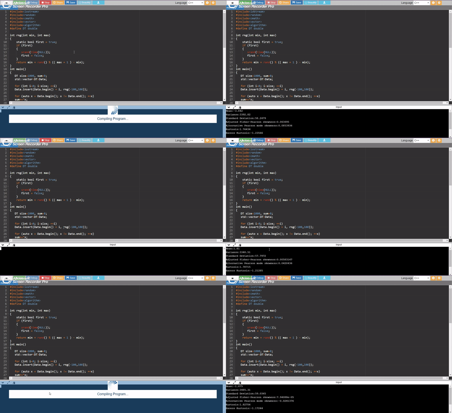
A few runs: (output)

| Anirban | 03/06/2020 |