Complexity classifiers

Following up with the complexity classification process as derived from GuessCompx, this post discusses the complexity classification functions, along with a bit on glms, the corresponding formulae involved, and how they eventually predict the correct complexity class.

It was initially focused on the time complexity classifier, but space/memory complexity (terms used interchangeably) goes hand-in-hand when we are dealing with the term ‘complexity’ in computer science, which is one reason why I felt the package might be incomplete if its classification was left unattended to, although it was not in our primary objective as per the initial idea as staged here.

A Future blog post on the generalized complexity classifier will cover additional aspects of the same in case one wishes to dive a little deeper and understand the functionality with additional details such as issues with the logic, and how to deal with them.

Function Details : Parameters

The function accepts a data frame which should ideally consist of two columns Timings/Memory usage and Data sizes, as returned by the timings-quantifying function/memory usage quantifying function.

Function Details : Implementation

A data frame containing the data sizes and time/memory results serves as input to fit different complexity models (logarithmic, linear, quadratic etc.) via several generalized linear models (glms) of the formula glm(time ~ (size_variation)), where size-variation can be ones such as (size) for linear time/memory, I(log(size)) for logarithmic, I(size^2) for quadratic etcetera.

The I() function here acts to convert the argument inside I(...) to as we expect it to be or work like, as in function formula where we need to explicitly inhibit the interpretation of formula operators so they can be used like regular arithmetical operators (such as the ^ used for exponentiation here) inside our glm() scope.

Note that the log-linear or NlogN complexity has a transformation involving the N variable twice (in N and logN respectively), for which an extra NlogN case was included throughout GuessCompx-code, since it could not be passed as a model formula and was in-turn required to be computed before passing it inside theglm() scope. Marc Agenis mentioned that this was one thing he was not happy about in his code when we were discussing the same. (I had doubts on the subject of the NlogN variable)

As a good thing in my package, both asymptoticTimeComplexityClass and asymptoticMemoryComplexityClass (the difference being the columnar values of the data frame accepted) do not create/have any separate case for NlogN or log-linear complexity, may it be a separate variable or a mutated instance. It works as expected since it classifies log-linear functions correctly.

Regarding the basis of distinction on which the best model or complexity-class is chosen, the cv. glm() function (from the package boot) plays a crucial role by returning a ‘delta’ (first shows the raw cross-validation and secondly shows the adjusted cross-validation estimate) from which we extract the second attribute, which gives us the adjusted leave-one-out error estimate for our timings. The adjustment is designed to compensate for the bias introduced by not using leave-one-out cross-validation.

Eventually, the leave-one-out mean squared error is computed for each model from which the least error demarks the best model or the best fit for the complexity class, with respect to other complexity classes. (which tend to have a larger error margin in contrast)

Function Details : Return value

Both the functions return a string signifying the complexity class, which falls in one of these complexities:
Constant, Linear, Log, Log-linear, Quadratic.

Usage

Collect the data frame obtained from asymptoticTimings/asymptoticMemoryUsage and pass it as a parameter to asymptoticTimeComplexityClass/asymptoticMemoryComplexityClass respectively, or chain the functions together:

# Shell sort example: (Log-linear time complexity)
df <- asymptoticTimings(sort(sample(1:100, data.sizes, replace = TRUE), method = "shell" , index.return = TRUE), data.sizes = 10^seq(1, 3, by = 0.5))
asymptoticTimeComplexityClass(df)
[1] "loglinear"
# PeakSegDP::cDPA example: (Quadratic time complexity)
asymptoticTimeComplexityClass(asymptoticTimings(PeakSegDP::cDPA(rpois(data.sizes, 1), rep(1, length(rpois(data.sizes, 1))), 3L), data.sizes = 10^seq(1, 4, by = 0.5))
[1] "quadratic"
# An example of allocating a vector of given sizes: (Linear space complexity)
df <- asymptoticMemoryUsage(vector(mode = "numeric", length = data.sizes), data.sizes = 10^seq(1, 3, by = 0.5))
asymptoticMemoryComplexityClass(df)
[1] "linear"
# Likewise, allocating a matrix of given sizes: (Quadratic space complexity)
asymptoticMemoryComplexityClass(asymptoticMemoryUsage(matrix(data.sizes:data.sizes, data.sizes, data.sizes), data.sizes = 10^seq(1, 5, by = 0.1)))
[1] "quadratic"

Diagnostic Plots

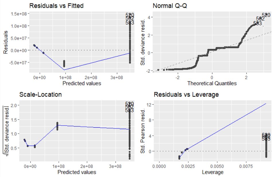
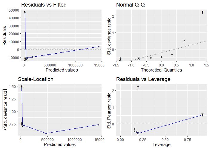
ggfortify, an extension of ggplot2, can be used to produce diagnostic plots for generalized linear models with the same formulae as used in the complexity classification process. For instance, we can use a linear predictor between Timings/Memory usage and Data sizes column to obtain visually comprehendible information on the predicted values:

library(ggfortify)
df.time <- asymptoticTimings(PeakSegDP::cDPA(rpois(data.sizes, 1), rep(1, length(rpois(data.sizes, 1))), 3L), data.sizes = 10^seq(1, 5, by = 0.5))
df.memory <- asymptoticMemoryUsage(PeakSegDP::cDPA(rpois(data.sizes, 1), rep(1, length(rpois(data.sizes, 1))), 3L), data.sizes = 10^seq(1, 5, by = 0.5))
glm.time.plot.obj <- glm(Timings~`Data sizes`, data = df.time)
glm.memory.plot.obj <- glm(`Memory usage`~`Data sizes`, data = df.memory)
ggplot2::autoplot(stats::glm(glm.time.plot.obj))
ggplot2::autoplot(stats::glm(glm.memory.plot.obj))

Code

• asymptoticTimeComplexityClass

  asymptoticTimeComplexityClass = function(model.df)
  { # Check for required columns as existent in the data frame produced by asymptoticTimings:
  if(class(model.df) == "data.frame" & "Timings" %in% colnames(model.df) & "Data sizes" %in% colnames(model.df))
  { # Create different glms of the formula (x(Timings) ~ y(Data sizes)) for our data frame and extract the fits in different variables signifying a complexity class each:
    constant   <- glm(Timings~1,                              data = model.df); model.df['constant'] = fitted(constant)  
    linear     <- glm(Timings~`Data sizes`,                   data = model.df); model.df['linear'] = fitted(linear)
    log        <- glm(Timings~log(`Data sizes`),              data = model.df); model.df['log'] = fitted(log)
    log.linear <- glm(Timings~`Data sizes`*log(`Data sizes`), data = model.df); model.df['log-linear'] = fitted(log.linear)
    quadratic  <- glm(Timings~I(`Data sizes`^2),              data = model.df); model.df['quadratic'] = fitted(quadratic)
    # Create a list:
    model.list <- list()
    # Loop through different complexity classes:
    for(complexity.class in c('constant', 'log', 'linear', 'loglinear', 'quadratic'))
    { # Collect the fitted values in a list with corresponding complexity names:
      model.list[[complexity.class]] = eval(as.name(complexity.class))
    }  
    # Apply cross validation on each glm in the list via a lapply on a function based on our data frame and extract the adjusted delta error: (second parameter)
    cross.validated.errors <- lapply(model.list, function(x) cv.glm(model.df, x)$delta[2])
    # Select the model with the least error as our complexity class:
    best.model <- names(which.min(cross.validated.errors))
    # Print it:
    print(best.model)
  }
  # Stop if specified columns don't exist: (i.e. the data frame passed is not in the format as returned by our timings quantifier)
  else stop("Input parameter must be a data frame with columns 'Timings' and 'Data sizes'")
  }
  

• asymptoticMemoryComplexityClass

  asymptoticMemoryComplexityClass = function(model.df)
  { # Check for required columns as existent in the data frame produced by asymptoticMemoryUsage:
  if(class(model.df) == "data.frame" & "Memory usage" %in% colnames(model.df) & "Data sizes" %in% colnames(model.df))
  { # Create different glms of the formula Memory-usage ~ Data-sizes (x ~ y) for our data frame and extract the fits in different variables signifying a complexity class each:
    constant   <- glm(`Memory usage`~1,                               data = model.df); model.df['constant'] = fitted(constant)
    linear     <- glm(`Memory usage`~`Data sizes`,                    data = model.df); model.df['linear'] = fitted(linear)
    log        <- glm(`Memory usage`~log(`Data sizes`),               data = model.df); model.df['log'] = fitted(log)
    loglinear  <- glm(`Memory usage`~`Data sizes`*log(`Data sizes`),  data = model.df); model.df['loglinear'] = fitted(loglinear)
    quadratic  <- glm(`Memory usage`~I(`Data sizes`^2),               data = model.df); model.df['quadratic'] = fitted(quadratic)
    # Create a list:
    model.list <- list()
    # Loop through different complexity classes:
    for(complexity.class in c('constant', 'log', 'linear', 'loglinear', 'quadratic'))
    { # Collect the fitted values in a list with corresponding complexity names:
      model.list[[complexity.class]] = eval(as.name(complexity.class))
    }  
    # Apply cross validation on each glm in the list via a lapply on a function based on our data frame and extract the adjusted delta error: (second parameter)
    cross.validated.errors <- lapply(model.list, function(x) cv.glm(model.df, x)$delta[2])
    # Select the model with the least error as our complexity class:
    best.model <- names(which.min(cross.validated.errors))
    # Print it:
    print(best.model)
  }  
  # Stop if specified columns don't exist: (i.e. the data frame passed is not in the format returned by our memory usage quantifier)
  else stop("Input parameter must be a data frame with columns 'Memory usage' and 'Data sizes'")
  }
  

  rxoygen-documented versions:

• testComplexity/R/AsymptoticTimeComplexityClass
• testComplexity/R/AsymptoticMemoryComplexityClass