“A study conducted in the mid-1900s sought to investigate the effect of feed type on chick weight. Newly hatched chicks were randomly allocated into six groups, and each group was given a different feed supplement. Their weights in grams after six weeks are given along with feed types.” - this is the description of the chickwts data set that is available to play with in base R.
data()
?chickwts
Recently, I went about investigating it as a means to experiment with my current understanding of statistical testing procedures. I started by constructing a data frame termed chickwts2, being derived from chickwts with the feed column recatogrized into feed.type, with three separate categories assigned:
chickwts2 <- data.frame(weight = chickwts$weight,
                        feed.type = fct_collapse(chickwts$feed,
                                                 animal.based = c('meatmeal', 'casein'),
                                                 seed.based = c('sunflower', 'linseed'),
                                                 bean.based = c('soybean','horsebean')))
head(chickwts2)
## weight feed.type
## 1 179 bean.based
## 2 160 bean.based
## 3 136 bean.based
## 4 227 bean.based
## 5 217 bean.based
## 6 168 bean.based
tail(chickwts2)
## weight feed.type
## 66 352 animal.based
## 67 359 animal.based
## 68 216 animal.based
## 69 222 animal.based
## 70 283 animal.based
## 71 332 animal.based
Then I re-ordered these three levels:
chickwts2$feed.type <- fct_relevel(chickwts2$feed.type, 'seed.based', 'bean.based', 'animal.based')
levels(chickwts2$feed.type)
## [1] "seed.based" "bean.based" "animal.based"
Considering how the data is, an appropriate hypothesis test would be a one-way (only one categorical variable for the data, which is the feed type) analysis of variance (ANOVA) test, as with respect to the different types of feed, I want to see how much the (average) chick weights differ, or if they differ at all (considering a significant margin of difference). The categorized data (groups based on the feed types) is a perfect fit for an ANOVA, as it would then help me to check if the (average) chick weights of each group differ or not.
Note that I’m still considering the chicks to remain as ‘chicks’, and hence I am not terming them as ‘chickens’, since their weights were recorded after only six weeks of growth. (meaning that they were only six weeks old at that time, considering the fact that the primary investigator of this study indeed did test this on newly hatched chicks as mentioned in the description)
Hypotheses?
The null hypothesis, in this case, is that the average weight (μ) of the chicks is equal for each feed type. Symbolically, I can represent this as:
H0 : μseed.based = μbean.based = μanimal.based
On the other hand, the alternative hypothesis would be that at least one of the feed types produces a significantly different average weight in the chicks, or that at least one of the means above would (significantly) differ from another. Based on pairwise comparisons, I can represent the alternative hypotheses symbolically:
Ha : μseed.based ≠ μbean.based
or μbean.based ≠ μanimal.based
or μanimal.based ≠ μseed.based
Assumptions
Two common assumptions in statistical inference procedures are the independence of the measurements and the sample’s representation of the population of interest. Neither of these assumptions appears to be explicitly addressed in the data description above, but I could ask a single question to the primary investigator of this study to assess the validity of these assumptions.
That question would be whether or not the data was actually collected from the chick population of interest via some form of sampling (such as SRS or stratified or clustered). This should be able to answer whether or not the sample represents the population of interest, which in our case would be chicks (or rather new-born chicks perhaps), taking into account a particular variant. For independence, I initially thought that this was mentioned, as the text provided does say that the group was ‘randomly allocated into six groups’, but I realized that does not necessarily imply that a form of random sampling was performed. Thus, I ask for that as a sub-part of my question to verify the sample’s independence, taking into account that the sample would be completely different from and independent of other samples.
Note that there are other assumptions three in total to be precise for my ANOVA test (the first of which relates to what is stated above):
1) Sample independence: I am assuming that the observations are independent both within and across groups. Without knowing how the experiment was performed, I cannot assure that some sort of random sampling was done for the observations to be independent, but I am assuming this to be true.
2) Sample normality: I am assuming that the distribution of the response variable (chick weight in this case) for each group should be normal. Note that I can’t apply the Central Limit Theorem (CLT) here since my sample sizes are less than thirty for each feed type. (To be precise, there are 23 observations for the animal-based feed type, and 24 observations for both seed-based and bean-based variants, accounted separately - all three of them being less than 30 each)
3) Variance Equality: I am assuming that the variances in between the three feed types are equal, which is a standard assumption for my ANOVA test (homoscedasticity).
Visualization & Normality Checks
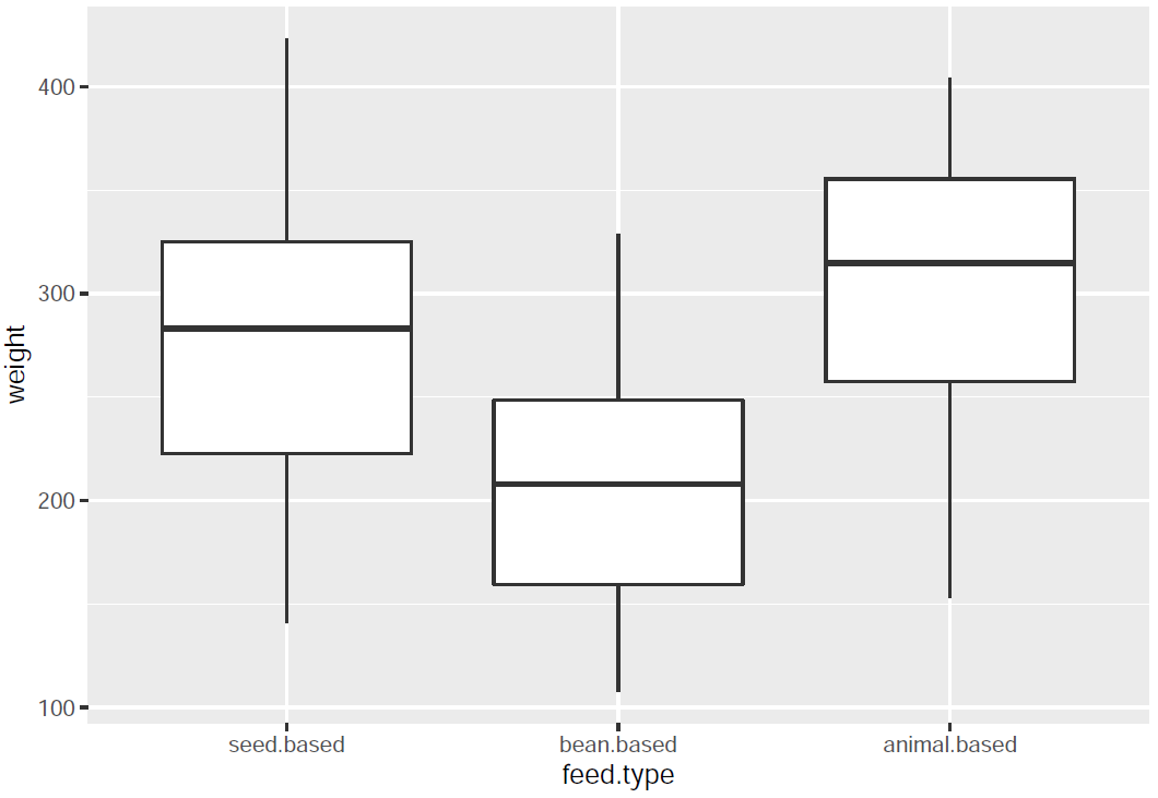
I create a boxplot to visualize the data (average chick weights) based on the feed type:
ggplot(chickwts2, aes(x = feed.type, y = weight)) + geom_boxplot()

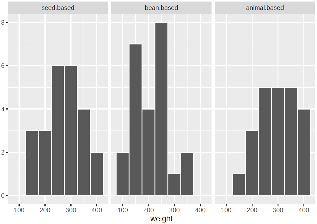
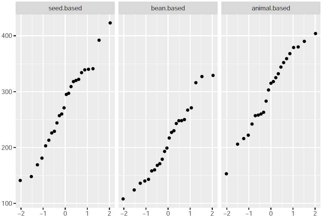
I proceed to create both a histogram and a QQ plot so as to visually discern if the distribution followed by a particular feed type pertains to the normal distribution (or is close enough to it):
qplot(x = weight, data = chickwts2, geom = "histogram",
      facets = ~ feed.type, color = I("white"), binwidth = 50)

As can be seen from the histograms, the seed-based feed type is close to a normal distribution, whereas the bean-based and the animal-based variants do not appear to resemble normal distributions all that well, although both could be normal, especially animal-based, given that the left side’s appearance resembles that of a perfect bell-shaped slope.
qplot(sample = weight, data = chickwts2, facets = ~ feed.type)

As for the QQ plots, the same observations can be made, with the seed-based feed type having the least amount of outliers and with most of its points (especially in between the first and third quantile) lying in a straight line, being indicative of a normal distribution pattern. As for the bean-based and animal-based variants, they have comparatively more outliers and the points are slightly more scattered than being in a straight line, implying that the distribution doesn’t resemble normality all that well, but it is possible that they are normal. Again, the animal-based distribution is better than the bean-based type (although not as good as the seed-based type), and resembles normality to some extent.
It’s hard to say a direct yes/no as to whether the assumption of normality is being violated, since the sample sizes are small, and for each group, they are less than 30. I would like to say that it is a yes for the bean-based feed type, and I’m also inclined to say the same for the animal-based seed type, since their distributions do not appear to be normal all that well, or if they do in fact are normal, it’s kinda stretchy (definitely not perfectly normal!). At the same time, I could say a no since the sample sizes are small, and may not be accurately reflective of the actual distribution. (again, I can’t apply the CLT, so I am more inclined towards the yes)
If we were to consider sub-hypothesis tests (tests within our hypothesis test i.e. within my ANOVA), I already did the informal tests with graphical/visual analysis of the histograms and QQ-plots above. The only thing left to do is a formal test, so I will go with a Shapiro-Wilk test for each of the three feed types:
seed.based.test <- chickwts2 %>% filter(feed.type == "seed.based") %>% select(weight)
shapiro.test(seed.based.test$weight)
##
## Shapiro-Wilk normality test
##
## data: seed.based.test$weight
## W = 0.97251, p-value = 0.7289
bean.based.test <- chickwts2 %>% filter(feed.type == "bean.based") %>% select(weight)
shapiro.test(bean.based.test$weight)
##
## Shapiro-Wilk normality test
##
## data: bean.based.test$weight
## W = 0.95598, p-value = 0.3631
animal.based.test <- chickwts2 %>% filter(feed.type == "animal.based") %>% select(weight)
shapiro.test(animal.based.test$weight)
##
## Shapiro-Wilk normality test
##
## data: animal.based.test$weight
## W = 0.9641, p-value = 0.5508
The null hypothesis that is being considered here is that the distribution for the particular feed type is normal. Depending upon the p-value thus obtained (greater than or less than 0.05, the standard alpha value to test against, at 95% confidence level), I will either accept or reject this hypothesis of mine.
From the Shapiro-Wilk tests that I conducted above, I get the p-value for the seed-based test to be 0.7289, which is clearly more than 0.05, indicating that I should accept my null hypothesis, which in turn implies that the seed-based feed type does indeed follow a normal distribution.
For the bean-based test, the p-value I obtained is 0.3631, which is more than 0.05, implying that I should not reject my null hypothesis, concluding that this variant of the feed type does pertain to normality too, although this isn’t very reassuring.
For the animal-based test, the p-value I obtained is 0.5508, which is more than 0.05, implying that I should not reject the null, and conclude that this variant of the feed type pertains to normality as well. Better than bean-based definitely, but still debatable.
I got the same conclusions from both my informal and formal sub-hypothesis tests for each of the three feed types, but I wouldn’t strictly emphasize that exists for all three of them based on the formal Shapiro-Wilk test, since it is known to be not good with small sample sizes.
Variance Equality Checks
Note that the assumption of homoscedasticity (equality of variances) hasn’t been addressed yet - i.e., I haven’t checked whether the variances in between the three feed types are equal or not. They should be equal in order for us to apply the ANOVA test. Let’s check that using some informal and formal procedures below.
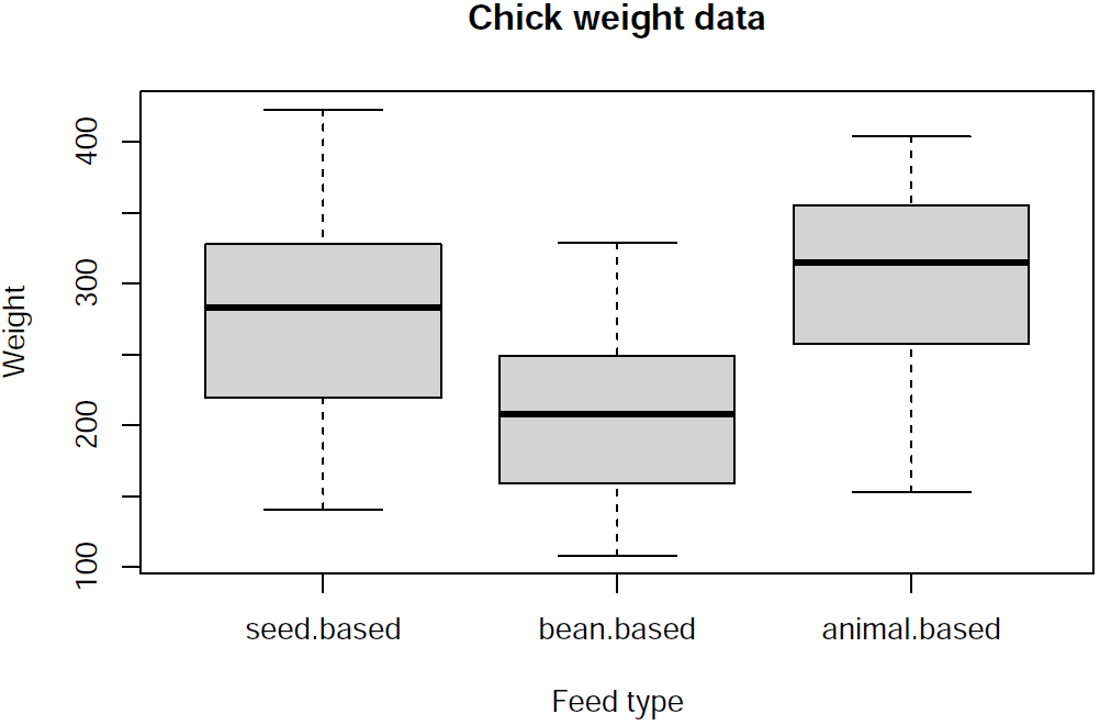
First, I create a boxplot to look at the measures of spread (such as range and IQR) and to visually discern if the variances are equal or not:
boxplot(weight ~ feed.type, chickwts2,
        main = "Chick weight data", xlab = "Feed type", ylab = "Weight")

By observing the box sizes, I notice that the interquartile range of all three of these feed types are about the same, and thus I can infer from this boxplot that the feed types have similar variations.
Note that this was an informal sub-hypothesis (within ANOVA) test to check for the equality of variance.
Now I conduct Levene’s test, which is a formal way to check for the same:
leveneTest(weight ~ feed.type, chickwts2)
## Levene’s Test for Homogeneity of Variance (center = median)
## Df F value Pr(>F)
## group 2 0.2969 0.7441
## 68
The above conducted Levene’s test results in a p-value of 0.7441, which is greater than 0.05 or even 0.01 (values for alpha at 95% and 99% confidence levels respectively), so I fail to reject the fact that the variances are equal, and I verify that this assumption (equality of variances) was indeed true. Thus, my ANOVA test too, in turn, is valid.
Given that all the assumptions for my test are being proven to be valid (normality and equality of variances, taking the independence of the sample’s observations to be granted), I can indeed say that performing an ANOVA as my hypothesis test was appropriate here. (satisfying assumptions fortify my aforementioned rationale)
Analysis of Variance
Proceeding to conduct my main hypothesis test, I fit a linear model for my data and then perform an ANOVA test on that:
chickwts2.model <- lm(weight ~ feed.type, data = chickwts2)
anova(chickwts2.model)
## Analysis of Variance Table
##
## Response: weight
## Df Sum Sq Mean Sq F value Pr(>F)
## feed.type 2 102433 51217 10.741 8.838e-05 ***
## Residuals 68 324252 4768
## ---
## Signif. codes: 0 ’***’ 0.001 ’**’ 0.01 ’*’ 0.05 ’.’ 0.1 ’ ’ 1
glance(chickwts2.model)$p.value
## value
## 8.837774e-05
I get a p-value of ~0.0000884, which is definitely way less than the standard alpha values of 0.05 (at 95% confidence level) and 0.01 (at 99% confidence level), indicating that the null hypothesis should be rejected.
The statistical conclusion here would be that the average chick weights differ and are not equal for each feed type, which implies that the feed type does indeed have an effect on chick weights, or rather chick growth - i.e. some are better, and some are comparatively less effective for chick growth, with the metric to measure that being the weight of the chicks.
Note that my conclusion above is more generalized and reflects upon whether the variants of the feed types did have an impact and therefore showed a statistically significant change in the chick weights or not in comparison to each other. It does not indicate which among the feed types showed significantly different average chick weights and as to which one is greater or lesser in a pairwise comparison, more specifically it does not answer such questions: “Does it indicate or support the idea that animal-based feed is associated with higher average chick weights, in comparison to the seed-based feed type?”
Pairwise Mean Comparisons
An auxiliary hypothesis test is required to concisely answer the question posed above, and ones of the same nature (i.e., pairwise mean comparisons).
I thought to go for a Tukey’s Honestly Significant Difference (HSD) test to see how the means differ in between the feed types. Note that in order to apply this, the equality of variances in between the feed types must be true, but I already checked and confirmed that in the variance equality checks section with both one informal and formal test (in addition, an informal var.test() could be done in between seed-based and animal-based types, but the grouping factor feed.type must be reduced to those two levels only, with the omission of the bean.based variant), so I’m good to proceed:
results <- emmeans(chickwts2.model, pairwise ~ feed.type)
results$emmeans
## feed.type emmean SE df lower.CL upper.CL
## seed.based 274 14.1 68 246 302
## bean.based 210 14.1 68 182 239
## animal.based 301 14.4 68 273 330
##
## Confidence level used: 0.95
The above conducted Tukey’s test shows a higher mean value for the animal-based feed type as compared to the seed-based feed type, indicating and supporting the statement that an animal-based feed is associated with higher average chick weights, in comparison to a seed-based feed.
results$contrasts[2]
## contrast estimate SE df t.ratio p.value
## seed.based - animal.based -27.4 20.1 68 -1.361 0.1779
The contrast between means for the seed-based vs. animal-based feed also has a p-value greater than 0.05 (or even 0.01), indicating that there is a significant difference between those two, which would be my conclusion here.
Stats is fun, ain’t it?
| Anirban | 11/10/2021 |